Engineering Design Problem: When we design, we would like to:

• Improve product or process quality
• Reduce life cycle costs
• Reduce development lead times

This can happen during the initial design phase or sometime during the product's life.

The design process starts by generating ideas – the functional performance of these ideas has to be verified.

There are two ways to verify an idea's functional performance:

• Physical testing of a prototype, the final product or process.
• Prediction of the performance of the product or process.

When to measure and when to simulate?
What is the best choice?  Generally, the answer depends on the system, its behaviour, and the required results.

As a general guideline: Simulate what is easy to simulate and measure what is easy to measure!

Generally, it is better to simulate when:

• Evaluating concepts - before prototypes - are available.
• Many different or very long load cases have to be evaluated.
• Required outputs are difficult or impossible to obtain.
• Measurement will be very expensive (landmine tests).

Simulation Can Assist During:

Initial product development (no product or prototype is available)
Allows the designer to:

• Make well-founded decisions early in the product development process.
• Test more ideas in less time.
• Understand how product behaviour is affected by different factors.
• Discover unexpected behaviour.
• Be sure the product fulfils demands.

Continual product Improvement (prototype or product is available)

• Optimise design solutions for the next product generation.
• Estimate product sensitivity to changes in, e.g., weather, wear, and ageing.
• Test dangerous situations.
• Understand product behaviour and factors that affect the behaviour at controlled repeated conditions.

Analysis Paralysis?

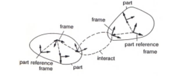
Model definition might be, according to Neelamkavil, "A model is a simplified representation of a system (or process or theory) intended to enhance our ability to understand, predict, and possibly control the behaviour of the system."

For testing or simulation, one of two approaches can be taken:

• Trial and error
  • This method is not well defined and can continue forever without providing any indication as to how close the design is to an optimal value.
• Testing programme, e.g., DOE study
  • More structured approach that gives the designer much more insight into how the design behaves.

MBD Simulation Methodology

1. Problem formulation
2. Definition of idealized model
3. Development of a computer model
4. Formulation of system equations
5. Equation solving
6. Results and post-processing
7. Evaluation and conclusion

1. Simulation Methodology: Problem formulation, describe:

• Technical problem to be solved
• Physical effects to include
• Limitations of the system
• System components
• Targets to achieve (force, torque, displacement..)

Design Example

1. Load cases
2. Bodies
3. Inverse Dynamics
   • Ideal constraints
4. Robust design
   • Model flexibility
5. Forward Dynamics
6. Model improvements
   • Door damper/closer
   • Automation

Design door

• Size: 0.6x2.0x0.04 (from ergonomic data)
• It must be comfortably operated by a standard human (see later for human force values).
• The door mechanism must be designed for infinite life.
• Design must be robust, e.g., not fail under limit manufacturing tolerances for automation.

Door V2

• Optimise door design
• Door add-ons
  • Damper
  • Opening mechanism

1. Design Example: Load Cases

• Own mass
• Opening Forces
• Extra accessories
• Manufacturing tolerances
• Misuse cases

2. MBD Simulation Methodology: Definition of idealised model

Collect relevant system data:

• Parts
• Component couplings (interactions between parts)

Model parameters

• Mass, centres of gyration, damping, stiffness

3. MBD Simulation Methodology: Development of a computer model driven by:

• Access to information
• Required results and accuracy
• Allowed simplifications
• Available resources (time and money)
• Model complexity
  • Static, quasi-static, Dynamic
  • 1D, 2D or 3D computer model
• Available modelling methods
  • Gravity
  • Rigid bodies
  • Ideal joints
  • Stiffness elements
  • Damping elements
  • General force components
  • Contact
  • Advanced elements (tyres, flexible bodies, ...).

Creating models in Adams/View

Location and Orientation

1. Points (Parametric): Location only
2. Markers: Location and orientation

Specifying Location and Orientation in Adams

• Location: specify in global or local coordinates
• Orientation: specify in global or local coordinates
  • Along Axis: Z-axis along the line of two points, arbitrary rotation.
  • In a plane: the Z-axis is along the line of the first two points; the third point locates the ZX-plane.

2. Design Example: Bodies

Part vs Geometry

• Good for concept evaluation
  • • Pendulum with out link

• Next step after acceptable results create CAD
  • • Pendulum with link

Parts In Adams

• All parts (except the ground part) have:
  • Initial position and orientation
  • Part mass & inertia
    • Mass and inertia reference
  • Initial velocities
  • Degrees of freedom
    • Governed by the laws of mechanics

Moment of Inertia Experiment

Participants:

• Blue -> Solid Cylinder
• Green -> Hollow cylinder
• Brown -> Solid Sphere
• Red -> Hollow Sphere

• The rolling radius of all participants is equal
• Mass for all participants is equal
• All participants roll without slipping

Constraints
Constraint equations in Adams

• Constraints are represented as algebraic equations in Adams/Solver.
• These equations describe the relationship between two markers.
• Joint parameters, referred to as I and J markers, define the location, orientation, and connecting parts:
  • The first marker, I, is fixed to the first part.
  • The second marker, J, is fixed to the second part.

Ideal Constraints in Adams

Joint Primitives in Adams

5. MBD Simulation Methodology: Equation solving

• Parameters:
• Solver type
  • Stiff methods (Implicit backwards difference formulations)
  • Non-stiff methods (explicit forward difference formulations)
• Step size
• Error
• Simulation duration

6. MBD Simulation Methodology: Results and post-processing

• Problem dependent
• Available tools
  • Time domain plots
  • Frequency domain plots
  • Animations
  • Data export

3. Design Example: Inverse Dynamics

Solve kinematic equations, but calculate the forces required to do so.
Use motions

• Joint motion
• Point motion

Measures: Your Virtual Instrumentation

• Predefined measures
  • Object
  • Point-to-Point
  • Included angle
  • Orientation
  • Range
• User-defined
  • Adams/view Computed
  • Adams/Solver function

7. MBD Simulation Methodology: Evaluation and conclusion

Compare system behaviour with the initial problem formulation

• Problem solved: continue to the next step in the development process
• Problem not solved: Find what is wrong, update and iterate the MBS procedure.
  • Unsatisfactory design
  • The model does not exhibit the required behaviour

Evaluate the certainty of results

• Assumptions
• Numerical approximation

Results Discussion

• Measures in local coordinate systems
• Redundant constraints: BAD! Why?
  • Indeterminate structure
  • Alternate constraint configuration

4. Design Example: Robust Design

• Manufacturing tolerance simulation
  Rotate hinge 0.1 deg.

Forces

• Forces for physicists:
  • Gravitation
  • Weak force
  • Strong force
  • Electromagnetic force

• Forces for engineers:
  • Body forces
    • Gravity
    • Electromagnetic forces
  • Aerodynamic forces
    • Buoyancy
    • Lift
    • Drag
    • Thrust
  • Contact or normal forces
  • Friction forces
  • Damping forces
  • Compliant forces (elastic)
  • Applied forces (push, pull, torque)
  • Fictitious forces
    • Coriolis force
    • Centrifugal force

Bushing

Adds linear flexibility

Flexibility: Where should the flexibility be added?

Results

Discussion

• The model is not overconstrained anymore.
• Forces increase with increasing angle of the bottom joint.
• Forces increase when the distance between joints reduces, but the effect of tolerance reduces?

5. Design Example: Forward Dynamics

Can a human open the door?

Applied Forces:

Figure 27: Applied forces

• Single Component Force
• Single Component Torque
• Torque Vector
• Force Vector
• General Force

Must select components, run time direction, and action and reaction bodies.

6. Design Example: Model Improvements

• Improve constraint model
  • Add play
  • Torque vs axial reaction forces
• Add a way of stopping the door when it is open and closed
  • Sensor
  • Stop torque
  • Point to plane contact
• Load prediction for finite element calculation
• Add a door damper to automatically close the door.

Back to Lecture Index