This blog is a bit overdue considering that the last blog on this topic was published at the end of 2019 and we are almost a quarter of the way through this year.
If you have forgotten what was discussed in Part 1 and Part 2, here is a quick recap of the main topics that were discussed.
In the first blog post the following topics were discussed:
- What is a y+ value?
- Laminar vs turbulent flow
- How to determine if your flow is laminar or turbulent?
- Introduction to wall functions
In the second blog post, the following topics were discussed:
- What is a boundary layer?
- What are the viscous sublayer, the buffer layer, and the log-law layer?
- What is a wall function?
- What are y+ and U+?
- What ranges of y+ should I target?
- How do I target a specific y+ value?
Now back to the present day and the topics that I plan to discuss during this blog.
The blog post will focus on the following topics:
- How to calculate the cell height adjacent to the no-slip wall to target a specific y+ value.
- Calculate the cell height of the cell adjacent to the no-slip wall.
- Approximate the shear stress at the no-slip wall.
- Calculating the skin friction coefficient
- A brief overview of the tutorial blog that will follow. Putting the theory into practice.
We are almost at a point where we have covered the basic theory behind the y+ value and targeting a specific y+ value. The last bit of theory that needs to be covered is how to make an initial guess on the cell size of the cell directly adjacent to the non-slip wall.
Once this last bit of theory is covered, we can move on to the more exciting stuff and implement this in practice.
How to calculate the wall-adjacent cell height to target a specific y+ value
The first step is to look at the quantities required to be able to approximate the required cell height for a specific y+ value. The equation to calculate the cell height is given by Equation 1:
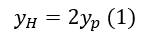
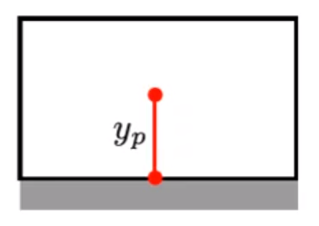
Figure 1: Cell Adjacent to the No-slip Wall
Where yp is given by Equation 2
- y+: Dimensionless distance to the wall
- yp: Distance normal to the wall where y+ is calculated
- U: Velocity parallel to the wall as a function of y
- Uτ: Shear velocity
- μ: Dynamic viscosity
- ρ: Density
The required fluid properties should be relatively easy to obtain, and the y+ value is the value that you would like to target for the specific turbulence model that you want to use.
The only unknown in Equation 2 is the shear velocity. From our previous discussions, we already know that the velocity at the no-slip wall is 0 m/s. We cannot use 0 m/s because y+ will be undefined, and in this case, the next best location to approximate the shear velocity is close to the wall.
In the case of most CFD (Computational Fluid Dynamics) packages, this location is at the centroid of the cell adjacent to the no-slip wall. The reason why the cell centroid is a particularly convenient location is because the Finite Volume Method is used to solve the Navier-Stokes equations, and the locations where the equations are solved are at the cell centroid.
Approximate the shear stress at the no-slip wall.
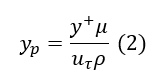
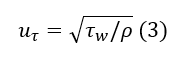
From previous discussions, we already know that the friction velocity is a function of the shear stress as given by Equation 3.
Where τw is given by Equation 4:
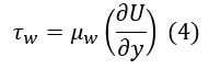
- τw: Shear stress
- μw : Dynamic wall viscosity
- U: Velocity parallel to the wall as a function of y
- y: Distance from thw wall
From our previous discussions we know that the turbulence models can quite easily determine the velocity gradient because we have two points where the velocity is known (y=0 and y=yp) but for an initial guess we only know the velocity at the wall.
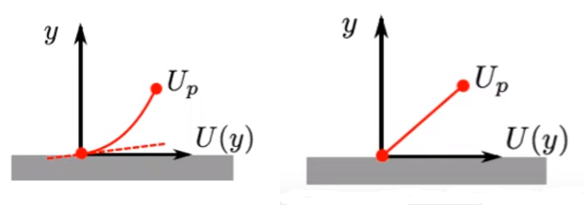
Figure 2: (L) High Reynolds Number (R) and Low Reynolds Number Solvers
This implies that we need an alternative way to approximate the wall shear stress. It is possible to get an approximation of the wall shear stress based on empirical data for different geometrical shapes.
The wall shear stress can be approximated by Equation 5
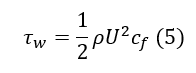
- cf: Skin friction coefficient
Calculating the skin friction coefficient
The skin friction coefficient can be calculated using various formulas depending on the geometry type. In general, the skin friction coefficient is calculated using Equation 6.
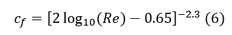
This skin friction coefficient is only valid for fully developed flow across a flat plate, so you can look for skin friction coefficients that are more applicable to your geometry. Remember this is only an initial guess, so using a different skin friction coefficient should not make too much of a difference.
The chances that your initial guess will give you the exact y+ value that you are targeting is relatively slim, but it will give you an indication of by how much you should increase or decrease your cell size adjacent to the no-slip wall to get closer to your targeted y+ value.
Online calculator
As you can see there are quite a few quantities that need to be calculated before you are able to calculate the cell size. Luckily, there are quite a few online calculators that can do this calculation for you.
The calculator that this blog is based on can be found at this website: https://www.fluidmechanics101.com/pages/tools.html

First Cell Height Calculator
The other calculators available should work more or less the same.
Remember, it might take a couple of iterations before you get to the y+ values that you are targeting. The calculator will just assist you with an initial guess for the cell height, but it is still better than just choosing random values.
Tutorial: Targeting a specific y+ value
In the next blog post, we will focus on putting the theory into practice using Cradle scFlow.
The aim of this tutorial is to go through:
- The basic steps to set up a CFD analysis using scFlow 2020.
- Octree settings
- Mesh and prism layer settings
- Solving the CFD simulation
- What information is available in the L-File
- Post-processing
- Getting the y+ distribution to see if the targeted y+ value was obtained
The tutorial would look at two examples as shown below.
Example 1: Flow in a straight pipe

Figure 3: Straight Pipe Example
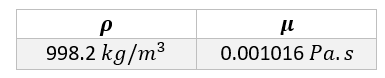
Table 1: Geometry Dimensions
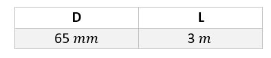
Table 2: Material Properties
The dimensions of the pipe have been chosen in such a way that the flow is fully turbulent at the inlet of the pipe. The pipe is also long enough for the flow to reach a fully developed state before it exits the pipe
Example 2: Flow in a pipe system
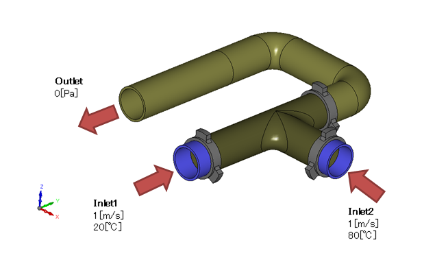
Figure 4: Pipe System Example
This geometry is the same as the geometry used in tutorial 1 of scFlow's operations examples. The same material properties will be used as in Example 1.
The information provided should be enough to allow you to do your own investigation but we will cover this in the next blog post
Stay tuned until next time.