The topic of targeting a specific y+ value for a turbulent flow simulation is a very important topic. There is however a bit of groundwork that needs to be done before being able to build a mesh to target a specific y+ value.
In this first part we will focus mainly on the following topics:
- What is a y+ value?
- Laminar vs turbulent flow.
- How to determine if your flow is laminar or turbulent?
- Introduction to wall functions that will be discussed in the next blog post.
If you are a computational fluid dynamics (CFD) expert or relatively new to the field, you should have read or hear of the y+ value. If you know exactly what the y+ value is and how to generate a mesh to target a specific y+ value this series of blog posts should refresh your memory and you might learn something new. If you are new to the field of CFD this series of blog posts should at least open your eyes to some of the pitfalls that you should watch out for.
What is a y+ value?
The y+ value is a non-dimensional distance. It is often used to describe how coarse or fine a volumetric mesh is for a flow pattern. It is important for the modelling of turbulence to determine the proper size of the mesh cells near no-slip walls.
From the definition of the y+ value there are two important things to note:
- It is only applicable to turbulent flow.
- It is applicable to the mesh cells directly in contact with a no-slip wall.
This also implies that laminar flow is not dependent on the y+ value which is correct. Laminar flow will be discussed as a separate topic in another blog post.
Laminar vs turbulent flow
A visual illustration of how the fluid flow over a flat plate develops is given in Figure 1. From this figure the flow can be categorised into three categories:
- Laminar flow
- Transition flow
- Turbulent flow
In most cases you will design your system to operate either in the laminar or turbulent region. The reason why we target the laminar or turbulent region is because we have equations based on empirical data to describe the behavior of the flow in those regions. The transition region is mainly avoided because there is a rapid change in the behavior of the flow and it is difficult to fit a curve to the empirical data to accurately model the behavior in this region.
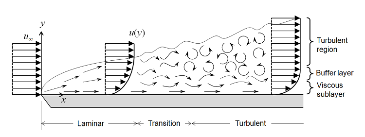
Figure 1: Development of Flow Over a Flat Plate
Laminar flow can be described as flow that moves in an orderly fashion in a specific direction whereas turbulent flow on the other hand is flow that moves in a disorderly fashion at different velocities and in different directions although the flow still moves in a specific direction. The difference flow patterns for laminar and turbulent flow are illustrated in Figure 2.
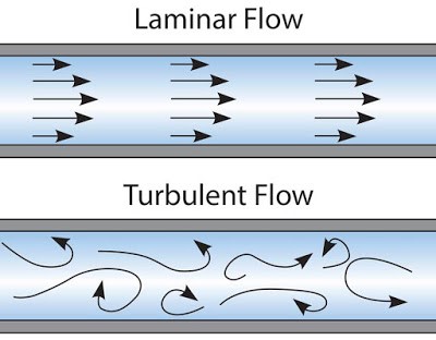
Figure 2: Laminar vs Turbulent Flow
It is possible to have regions of predominantly laminar and predominantly turbulent flow in a single application. What do you do in this scenario? You need to identify the region that you are interested in to drive your flow type selection. An example of this is given in Figure 3. The flow in the bottom half of the figure (Green rectangle) is predominantly laminar and the flow in the top half of the figure (Red rectangle) is predominantly turbulent.
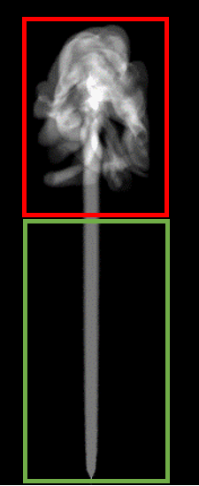
Figure 3: Smoke from an Incense Stick
How to determine if the flow is laminar or turbulent
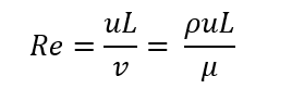
Everyone should know how to determine if the flow is turbulent or not if you had some type of flow course in varsity but if you have forgotten how, it is done by calculating the Reynolds number of the flow being analyses.
 where:
- Re is the Reynolds of the flow
- ρ is the density of the fluid (kg/m3)
- u is the velocity of the fluid (m/s)
- L is a characteristic length (m) = ~ the system Volume divided by the area
- μ is the dynamic viscosity of the fluid (Pa·s or N·s/m2 or kg/m·s)
- v is the kinematic viscosity of the fluid (m2/s).
Once the Reynolds number is calculated it is possible to determine if the flow is in the laminar transition or turbulent region based on limits obtained from empirical data.
When determining the flow type it is important to ensure that you calculate the Reynolds number using the correct characteristic length and velocity based on the empirical data being used. In the case of a cylinder the velocity will be the free-stream velocity and the characteristic length will be the diameter.
Usually the Reynolds number is calculated at the inlets of the fluid domain as the fluid velocities are usually known at the inlets. Remember the Reynolds number gives an indication if the flow is laminar, in transition or turbulent at the location where it is calculated but that does not mean that it is a good assumption for the whole domain. It is always a good idea to check the velocity profile after you have completed the analysis to see if the assumption is indeed valid for the fluid domain and the flow is predominantly laminar or predominantly turbulent. The laminar and turbulent velocity flow profiles should look something like the illustration in Figure 4.
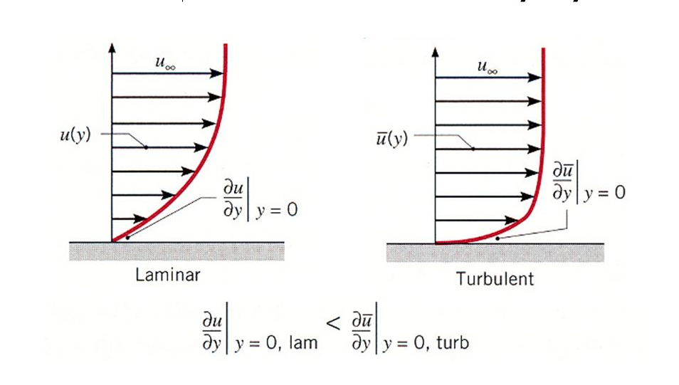
Figure 4: Velocity Profiles of Laminar and Turbulent Flow
Now that we know how to determine if the flow it turbulent or not, we can move on to why the y+ value is applicable to fluid cells directly in contact with the no-slip wall and why we are interested in the areas close to the wall.
In any flow analysis one of the quantities that we are interested in, is the velocity of the fluid or more specifically the velocity profile of the fluid. Any place where a moving fluid meets a wall with a no-slip condition a velocity profile as show in Figure 4 will be created. This is more commonly known as the flow boundary layer.
It is clear from Figure 4 that a high velocity gradient is created as the velocity increases from 0 m/s at the no-slip wall to the free stream velocity far away from the wall. It is exactly in the regions of the high velocity gradients where we cannot use momentum equations to calculate the velocity and we required a different way of calculating the velocity profile in these regions and this is where the y+ value comes into play.
The functions used to describe the velocity in the regions of high velocity gradients close to the no-slip wall in terms of the y+ value is known as a wall functions. The wall functions are based on the empirical date and is given in Figure 5.
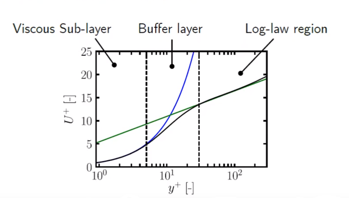
Figure 6: Wall Functions
Wall functions (Figure 5) will be discussed in detail in the next blog post, and you are more than welcome to read up on wall functions in the meantime. As a starting point I will recommend that you start by watching the video below by Dr Aidan Wimshurst.
https://www.youtube.com/watch?v=fJDYtEGMgzs?rel=0